Anomaly Detection for Non-Normal Data

Unsupervised, Multivariate Statistical Anomaly Detection for Data with Complex Distributions

Anomaly detection is a field within machine learning that has been thoroughly explored, with methods from k-nearest neighbor to isolation forests to clustering. But what if we want to limit our anomaly detection to statistical methods only? Furthermore, what if our data doesn’t follow parametric distributions?

At Okaya, we deal with a wide myriad of clients, from firefighters to students to veterans. It’s important to capture the differences between these many groups. For example, with respect to something like sleep time, a firefighter working the night shift will have drastically different sleep and wake times compared to someone like a student. How can we capture these relationships and make statistical inferences on those relationships?

Parametric Statistical Modeling

Why might we want to limit our methods to statistical methods only? There are two main reasons:

1. The ability to calculate a probability for a test point as to whether it is an anomaly or not. This allows us to easily set anomaly thresholds.
2. Superior computation speed. Since statistical modeling relies on distributions for which libraries for fast, easy calculation already exist, it is relatively simple to implement an algorithm that runs quickly.

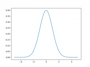
One of the most commonly used and commonly taught statistical methods makes use of the normal curve.

As a review, recall that the normal curve has mean μ and standard deviation σ, for which μ defines where the curve is centered, and σ defines how spread apart our distribution is.

Essentially, what we are going to do is fit our data to a normal curve, resulting in parameters μ and σ which fit our input dataset. Once we have these values, we can easily calculate a probability density value from any given test input. This represents a “probability” of that test input being an anomaly or not (that is, the lower the probability, the higher the likelihood of it being an anomaly).

vision Image

Non-Parametric Statistical Modeling – Motivation

However, we are making a dangerous assumption when we assume our data fits the normal curve (or any other statistical distribution, for that matter). It is true that we can use the central limit theorem (CLT) in many situations, and thus approximate a distribution to be normal. But what if we are actually relying on data to not fit to a normal curve? CLT only works across large populations – however, at Okaya, we are aiming to personalize data analysis instead.

The Kernel Density Estimator

Essentially, what we’d like is a statistical distribution that follows whatever shape the input data represents. Intuitively, wherever there is more data, we would expect the distribution to be more dense at that point.

We will use an example dataset of sleep lengths (in hours):

firefighter_sleep_lengths = [5, 5.5, 4.7, 5.6, 6.2, 5.4, 5.7, 4.3, 4.9]
student_sleep_lengths = [8.3, 8.1, 7.9, 8.5, 8.6, 8.4, 8.9, 9]

from scipy.stats import multivariate_normal

input_data = firefighter_sleep_lengths + student_sleep_lengths
kernels = []

for point in input_data:
    kernels.append(multivariate_normal(point))
Multivariate Non-Parametric Modeling
In today’s data-centric world, we can gain even more information by using multivariate data. When we use statistical distributions that are solely based on the magnitude of input data (for example, sleep length), we are assuming these numbers are random variables. However, data is hardly ever truly random. We would expect a variety of factors to have an influence on what our data looks like.

The methodology for calculating probabilities is exactly the same as before, except we put in 2 numbers for the input mean of the multivariate normal, instead of just 1 like before.

Making Use of Features
Though we can make use of featured data to make more nuanced anomaly detections, we can also use features to make more powerful predictions. We might be interested in calculating an expected value, in which we input a number of features and return an expected value that has been calculated based on those features.

python
Always show details

Copy code
def predict(kernels, test_point):
    probs = []
    for kernel in kernels:
        probs.append(kernel.pdf(test_point))
    return sum(probs) / len(probs)
Conclusion
The importance of non-parametric modeling is not to be ignored. To achieve this goal, we use kernel density estimation to capture more complex relationships which parametric curves such as the normal distribution cannot model. This allows us to make more accurate predictions and detect anomalies more effectively.

References
Normal distribution
Kernel density estimation
Central limit theorem